Choropleth maps in R
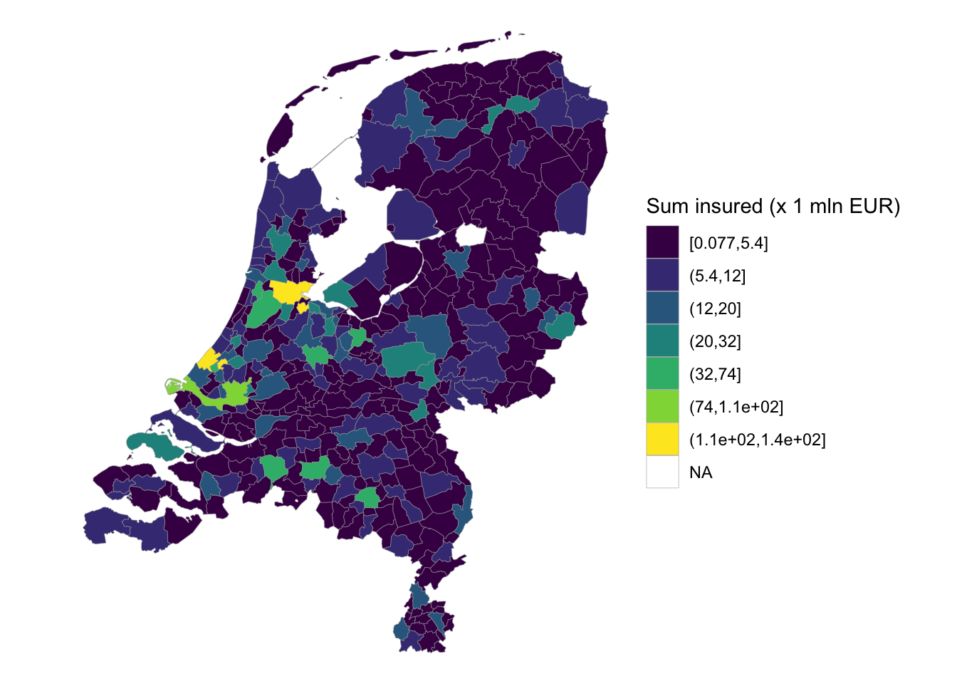
The goal of this post is to show how to create choropleths of the Netherlands in R. Typically in R it is difficult to create choropleths. One main problem is on merging the names in the shapefile with the names used in the data set. For example, in case of municipality names in the Netherlands it is common that due to municipal reorganizations or due to punctuation marks in municipality names it is not easy to merge the municipality names in the shapefile with the names in the data set. To elegantly solve this problem the choropleth maps are not shaded based on a value for a region but directly on the points within that region. The general idea is to convert both the point data and polygon data to spatial objects. After that, count how many points fall within that polygon. This method is illustrated by an insurance data set. The insurance data set contains of 20,000 postal codes with a sum insured and given coordinates. The goal is to shade a choropleth map with the total sum insured per municipality.
The above is possible using the sp package, which is
widespread and well-known in the R community, but I decided to use the
sf package because sf would be the next
generation standard of spatial objects in R (https://cran.r-project.org/web/packages/sf/index.html).
It implements a formal standard called “Simple Features” (see Wikipedia)
that specifies a storage and access model of spatial geometries (point,
line, polygon). A feature geometry is called simple when it consists of
points connected by straight line pieces, and does not intersect itself.
This standard has been adopted widely, not only by spatial databases
such as PostGIS, but also more recent standards such as GeoJSON. Knowing
the usage and functionality of sf will probably be
beneficial.
Reading a shapefile
The first step is to read the shapefile of the Netherlands on the
municipality level. There are different ways one can load a shapefile
into R. A quick benchmark shows the function st_read() from
sf does read much, much more quickly compared to the common
used function readOGR() from rgdal. Note that
shapefiles consist of more than one file, all with identical basename,
which reside in the same directory.
The function st_read() from sf is used to
load the shapefile.
library(sf)
#library(rgdal)
library(dplyr)
nl_gemeente_read <- st_read("data/nl_gemeente_2018/nl_gemeente_2018.shp",
quiet = TRUE)Let’s check the contents of this simple feature object. The short report printed gives the geometry type, mentions that there are 380 features (records, represented as rows) and 3 fields (attributes, represented as columns). Each row is a simple feature: a single record, or data.frame row, consisting of attributes and geometry.
nl_gemeente_read## Simple feature collection with 380 features and 3 fields
## Geometry type: MULTIPOLYGON
## Dimension: XY
## Bounding box: xmin: 13565.4 ymin: 306846.2 xmax: 278018.3 ymax: 619191.8
## Projected CRS: Amersfoort / RD New
## First 10 features:
## id code gemeentena geometry
## 1 1 0584 Oud-Beijerland MULTIPOLYGON (((85710.65 42...
## 2 18 0160 Hardenberg MULTIPOLYGON (((239027.4 52...
## 3 19 0327 Leusden MULTIPOLYGON (((161442.9 46...
## 4 20 1931 Krimpenerwaard MULTIPOLYGON (((107027.9 44...
## 5 21 1701 Westerveld MULTIPOLYGON (((204348 5410...
## 6 22 0689 Giessenlanden MULTIPOLYGON (((123137 4280...
## 7 23 1700 Twenterand MULTIPOLYGON (((227237 4975...
## 8 24 0373 Bergen (NH.) MULTIPOLYGON (((104965.5 53...
## 9 25 1525 Teylingen MULTIPOLYGON (((91850.13 46...
## 10 2 0448 Texel MULTIPOLYGON (((122420.6 56...For each row a single simple feature geometry is given. The above printed output shows that geometries are printed in abbreviated form, but we can view a complete geometry by selecting it, e.g. the first one by:
nl_gemeente_geom <- st_geometry(nl_gemeente_read)
nl_gemeente_geom[[1]]## MULTIPOLYGON (((85710.65 426642.1, 86755.6 427428.4, 88214.2 427221, 89200.6 428037.9, 90406.6 427480, 90281.87 426462.5, 90521.39 425252.7, 89346.33 424973.1, 89025.12 425085.8, 88884.43 423304.3, 88577.54 422352.4, 87852.2 421612, 86530.7 422211.5, 86445.2 422566, 85423.58 422572, 85728.09 424192, 86087.61 424151.5, 86109.93 425705.5, 85744.77 426084.9, 85710.65 426642.1)))The way this is printed is called well-known text, and is part of the standards. The word MULTIPOLYGON is followed by three parenthesis, because it can consist of multiple polygons, in the form of MULTIPOLYGON(POL1,POL2), where POL1 might consist of an exterior ring and zero or more interior rings, as of (EXT1,HOLE1,HOLE2)
Convert the coordinate reference system of the simple feature object
from NA to WGS84. The second line makes invalid geometries valid. This
can also be done using lwgeom::st_make_valid(x).
nl_gemeente_wgs84 <- nl_gemeente_read |>
st_buffer(0) |> # Make invalid geometries valid
st_transform(crs = 4326) |> # Convert coordinates to WGS84
mutate(id = row_number()) # Add column with id to each municipalityReading insurance data
This example uses insurance data. The data shows the sum insured for 20,000 postal codes in the Netherlands. The goal is to aggregate this sums on the municipality level. Therefore for each point in this data set we should find the corresponding polygon. The polygons are shaded according to the sum of the amounts within the boundaries of the polygon.
spatialrisk::insurance## # A tibble: 29,990 × 5
## postcode population_pc4 amount lon lat
## <chr> <dbl> <dbl> <dbl> <dbl>
## 1 2215KK 15385 20000 4.48 52.2
## 2 5296NS 2165 154965 5.29 51.6
## 3 3055CD 7955 146078 4.50 52.0
## 4 9665NM 8050 129304 7.00 53.1
## 5 2282CX 10320 67636 4.34 52.1
## 6 1187CM 17905 29971 4.83 52.3
## 7 1074HE 8320 20000 4.91 52.4
## 8 7944LD 9360 115893 6.18 52.7
## 9 3404CL 10275 110280 5.04 52.0
## 10 8266CP 6660 122500 5.92 52.5
## # ℹ 29,980 more rowsConvert points to a simple feature object. Note that the argument
crs (coordinate reference system) should be the same EPSG
code as above.
insurance_sf <- st_as_sf(spatialrisk::insurance, coords = c("lon", "lat"), crs = 4326) Merge sf objects
In the next step we merge the simple feature objects. The function
sf::st_join can be used to do a spatial left or inner join.
See documentation ?st_join on how to carry out an inner join.
insurance_map_sf <- nl_gemeente_wgs84 |> st_join(insurance_sf)
insurance_map_sf## Simple feature collection with 29972 features and 6 fields
## Geometry type: GEOMETRY
## Dimension: XY
## Bounding box: xmin: 3.358378 ymin: 50.75037 xmax: 7.227389 ymax: 53.55364
## Geodetic CRS: WGS 84
## First 10 features:
## id code gemeentena postcode population_pc4 amount geometry
## 1 1 0584 Oud-Beijerland 3262RD 9035 25000 POLYGON ((4.382132 51.82408...
## 1.1 1 0584 Oud-Beijerland 3262AA 9035 29971 POLYGON ((4.382132 51.82408...
## 1.2 1 0584 Oud-Beijerland 3262PL 9035 63389 POLYGON ((4.382132 51.82408...
## 1.3 1 0584 Oud-Beijerland 3262VC 9035 222958 POLYGON ((4.382132 51.82408...
## 1.4 1 0584 Oud-Beijerland 3262ES 9035 92800 POLYGON ((4.382132 51.82408...
## 1.5 1 0584 Oud-Beijerland 3263PC 5010 86464 POLYGON ((4.382132 51.82408...
## 1.6 1 0584 Oud-Beijerland 3261TD 9805 102402 POLYGON ((4.382132 51.82408...
## 1.7 1 0584 Oud-Beijerland 3262BG 9035 30000 POLYGON ((4.382132 51.82408...
## 1.8 1 0584 Oud-Beijerland 3262XR 9035 25355 POLYGON ((4.382132 51.82408...
## 1.9 1 0584 Oud-Beijerland 3261JJ 9805 122500 POLYGON ((4.382132 51.82408...Note the message
although coordinates are longitude/latitude, st_intersects assumes that they are planar.
Depending where you are on the globe, and the distance between points
forming a line or polygon, an apparently straight line in geographical
coordinates will be more or less curved when projected to the plane, but
for our use case (small area not near the poles) the message is of
little importance.
Next the object should be aggregated on the id column. Note that the
easiest would be to use the group_by and summarize statements directly
to the above sf object. It turns out that this approach
takes hours (see issue: https://github.com/r-spatial/sf/issues/661). To overcome
this it is better to perform the aggregation on a data.frame. This is
done by transforming the data from an sf object to a
data.frame (by removing geometries).
# Change from sf to data.frame
insurance_map <- insurance_map_sf
st_geometry(insurance_map) <- NULL
# Aggregate
insurance_map_sf0 <- insurance_map |>
summarize(output = sum(amount), .by = c(id))
insurance_map_sf2 <- left_join(nl_gemeente_wgs84, insurance_map_sf0) ## Joining with `by = join_by(id)`class(insurance_map_sf2)## [1] "sf" "data.frame"Note that joins also work when a data frame is the first argument. This keeps the geometry column but drops the sf class, returning a data.frame object.
Printing choropleths
Using ggplot2
ggplot2 is undoubedly the most popular package for
producing choropleths in R, and very powerful. It is used for all sorts
of plotting like the base graphics package, and unlike tmap is not
designed solely for mapping.
The geom_sf function is used to visualise simple feature (sf) objects.
library(ggplot2)
library(insurancerating)
library(viridis)
insurance_map_sf2_cut <- insurance_map_sf2 |>
mutate(output_cut = insurancerating::fisher(output / 1e6, n = 7))
ggplot(insurance_map_sf2_cut) +
geom_sf(aes(fill = output_cut), size = .1, color = "grey65") +
scale_fill_viridis_d() +
theme_void() +
labs(fill = "Sum insured (x 1 mln EUR)")
Using tmap
The following code shows another package for mapping simple feature
objects. tmap is my favourite for making maps (and also
very underrated). It has similar syntax to the popular ggplot2 but will
also produce a reasonable map with only a couple of lines of code.
library(tmap)
tmap_mode("plot")
tm_shape(insurance_map_sf2) +
tm_polygons(
"output",
id = "gemeentena",
fill.scale = tmap::tm_scale_intervals(style = "fisher",
values = "viridis",
n = 5),
fill.legend = tmap::tm_legend(title = "Insurance (in euros)"),
lwd = .1
) +
tm_compass(position = c("right", "bottom")) +
tm_scalebar(position = c("left", "bottom")) +
tm_style("gray")
It is easy to obtain the same map in html.
library(stringi)
insurance_map_sf2$gemeentena <- stringi::stri_encode(insurance_map_sf2$gemeentena, "", "UTF-8")
tmap_mode("view")## ℹ tmap mode set to "view".tm_shape(insurance_map_sf2) +
tm_polygons(
"output",
id = "gemeentena",
fill.scale = tmap::tm_scale_intervals(style = "fisher",
values = "viridis",
n = 5),
fill.legend = tmap::tm_legend(title = "Insurance (in euros)"),
lwd = .1,
fill_alpha = .5
)Data on shapefile level
In many problems it is common to have the data already on the level of the polygons in the shapefile. For example it could be possible that the sum insured per postal code is known. The following example shows how to plot this data set on a choropleth map on the postal code level.
pc_level0 <- spatialrisk::insurance |>
mutate(pc4 = as.numeric(stringr::str_sub(postcode, 1, 4))) |>
summarize(amount = sum(amount), .by = c(pc4))
pc_level <- left_join(spatialrisk::nl_postcode4, pc_level0)
tmap_mode("view")
tm_shape(pc_level) +
tm_polygons(
"amount",
id = "areaname",
fill.scale = tmap::tm_scale_intervals(style = "fisher",
values = "viridis",
n = 5),
fill.legend = tmap::tm_legend(title = "Insurance (in euros)"),
lwd = .1,
fill_alpha = .5
) Create new polygons
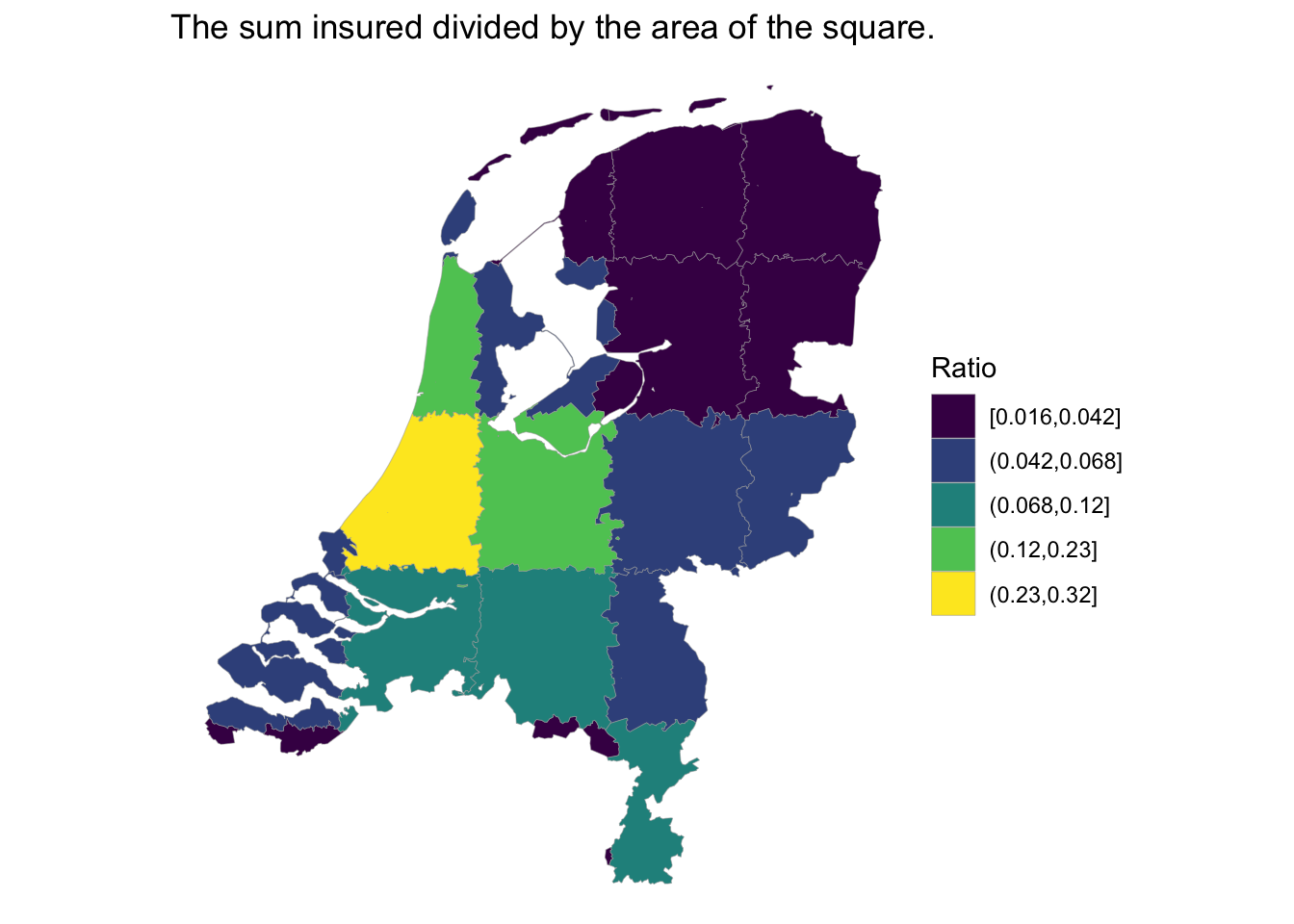
Note that approaching data from a small-area spatial perspective poses challenges. The way the municipalities are defined, such as their shapes and boundaries, is arbitrary and may be to large and undifferentiated to the spatial distribution of the sum insured. Therefore, municipalities may more properly be thought of as convenient ’bins’ into which the sums are gathered, rather than as objects of interest in themselves. It may be interesting to create choropleth maps at finer geographical resolutions. The following example shows how to create new polygons. The map shows a ‘patchwork’ pattern.
pc_level_nw <- st_make_valid(pc_level)
cent <- st_geometry(pc_level_nw) |> st_centroid() |> st_coordinates()
blocks_level <- pc_level_nw |>
mutate(area = as.numeric(st_area(pc_level_nw)), longitude = cent[,1], latitude = cent[,2]) |>
group_by(cut(longitude,5), cut(latitude,5)) |>
summarise(area = sum(area),
amount = sum(amount, na.rm = TRUE),
dens = mean(amount / area)) |>
ungroup() |>
mutate(denscut = insurancerating::fisher(dens, n = 5)) |>
filter(!is.na(denscut))
ggplot(blocks_level) +
geom_sf(aes(fill = denscut), size = .1, color = "grey65") +
scale_fill_viridis_d() +
theme_void() +
labs(fill = "Ratio",
title = "The sum insured divided by the area of the square.")