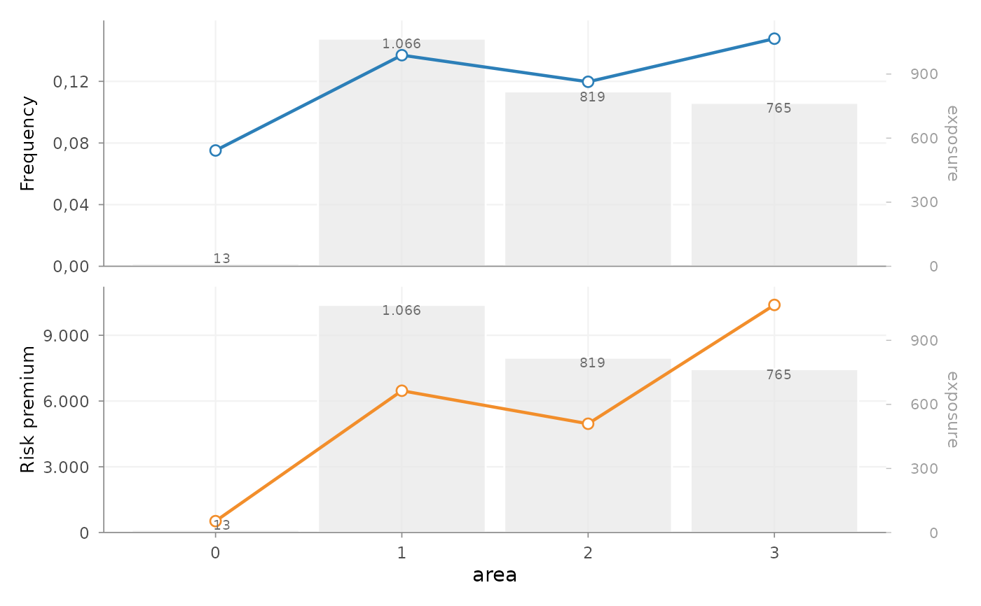
Aggregate observed claim, exposure and premium experience for one or more discrete risk factors. The result supports exploratory pricing analysis by showing how portfolio volume and unadjusted actuarial metrics vary across factor levels.
Usage
factor_analysis(
  data = NULL,
  risk_factors = NULL,
  claim_amount = NULL,
  claim_count = NULL,
  exposure = NULL,
  premium = NULL,
  group_by = NULL,
  df = NULL,
  x = NULL,
  severity = NULL,
  nclaims = NULL,
  by = NULL
)
Arguments
- data
A data frame containing portfolio observations.
- risk_factors
Non-empty character vector naming the discrete risk factors to analyse.
- claim_amount
Optional character string naming the total claim-amount column.
- claim_count
Optional character string naming the claim-count column.
- exposure
Optional character string naming the exposure column.
Optional character string naming the premium-amount column.
- group_by
Optional character vector naming additional grouping variables, such as underwriting year or product segment.
- df, x, severity, nclaims, by
Deprecated argument names. Use
data,risk_factors,claim_amount,claim_count, andgroup_byinstead.
Value
A data frame with classes "factor_analysis", "univariate" and
"data.frame". It contains the grouping columns, aggregated input columns
and all actuarial measures supported by the supplied inputs. The original
column names are retained for claim amount, claim count, exposure and
premium.
Details
Calculated measures
Depending on the supplied columns, the function calculates:
frequency = claim_count / exposure;average_severity = claim_amount / claim_count;risk_premium = claim_amount / exposure;loss_ratio = claim_amount / premium;average_premium = premium / exposure.
Input amount columns are summed before ratios are calculated. A measure is
omitted when its required inputs were not supplied. A zero or missing
denominator produces NA_real_ rather than an infinite value.
Actuarial interpretation
These are observed, univariate or stratified portfolio measures. They are not adjusted for correlation between rating factors and should not be interpreted as conditional GLM effects. Differences between levels may reflect portfolio mix, small exposure, claim volatility or changes over time. Claim counts, exposure and stability should therefore be reviewed alongside the ratios.
group_by can be used to compare the same risk-factor pattern across
periods or portfolio segments. autoplot.factor_analysis() provides the
corresponding graphical review. Modelled effects can subsequently be
inspected with rating_table().
Column interface
Column names are supplied as character strings. Deprecated univariate()
remains available for compatibility with its former interface.
Examples
area_experience <- factor_analysis(
  MTPL2,
  risk_factors = "area",
  claim_amount = "amount",
  claim_count = "nclaims",
  exposure = "exposure",
  premium = "premium"
)

area_experience
#>   area  amount nclaims   exposure premium  frequency average_severity
#> 1    2 4063270      98  818.53973   51896 0.11972540         41461.94
#> 2    3 7945311     113  764.99178   49337 0.14771401         70312.49
#> 3    1 6896187     146 1065.74795   65753 0.13699299         47234.16
#> 4    0    6922       1   13.30685     902 0.07514927          6922.00
#>   risk_premium loss_ratio average_premium
#> 1    4964.0474  78.296400        63.40071
#> 2   10386.1390 161.041632        64.49350
#> 3    6470.7486 104.880188        61.69658
#> 4     520.1832   7.674058        67.78464
autoplot(area_experience, metrics = c("frequency", "risk_premium"))