insurancerating provides actuarial tools and building blocks for analysing, modelling, refining, and validating insurance rating models in R.
The package is designed around common GLM-based pricing tasks and focuses on the translation of statistical model output into interpretable and controllable tariff structures.
Scope
The package supports common tasks that often occur in actuarial pricing work:
- exploratory analysis of risk factors
- estimation of GLM-based pricing models
- controlled refinement of model coefficients
- construction and interpretation of tariff structures
- evaluation of model performance and stability
The focus is on reproducibility, interpretability, and consistency across models.
Installation
Install the CRAN version:
install.packages("insurancerating")Or development version:
# install.packages("remotes")
remotes::install_github("MHaringa/insurancerating")
Quick example
library(insurancerating)
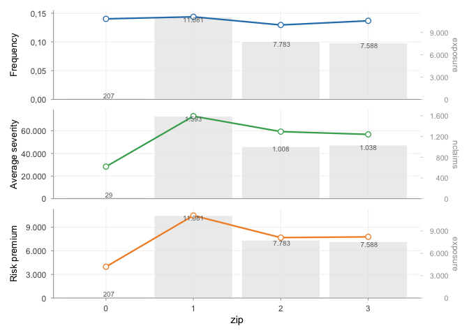
# Factor analysis
fa <- factor_analysis(
MTPL,
risk_factors = "zip",
claim_count = "nclaims",
exposure = "exposure",
claim_amount = "amount"
)
autoplot(
fa,
metrics = c("frequency", "average_severity", "risk_premium")
)
# Fit model
mod <- glm(
  nclaims ~ zip,
  offset = log(exposure),
  family = poisson(),
  data = MTPL
)

rating_table(mod)
## risk_factor level est_mod
## 1 (Intercept) (Intercept) 0.1402024
## 2 zip 0 1.0000000
## 3 zip 1 1.0254064
## 4 zip 2 0.9238016
## 5 zip 3 0.9757522
# Refine coefficients
zip_df <- data.frame(
  zip = c("0", "1", "2", "3"),
  zip_adj = c(0.90, 0.95, 1.00, 1.10)
)

mod_refined <- prepare_refinement(mod) |>
  add_restriction(zip_df) |>
  refit()

rating_table(mod_refined)Combining Building Blocks
A possible sequence of steps is:
factor_analysis()      # analyse portfolio
glm()                  # estimate model
prepare_refinement()   # apply adjustments
rating_table()         # interpret coefficients
Core components
Factor analysis
factor_analysis() provides aggregated portfolio metrics such as:
- frequency
- average severity
- risk premium
- loss ratio
These are used to assess the behaviour and credibility of risk factors.
Rating models
Models are estimated using widely used GLM specifications:
- Poisson for frequency
- Gamma for severity
- Gamma (log-link) for premium
rating_table() expresses model output in terms of original factor levels.
Refinement
Model output can be adjusted using:
prepare_refinement(model) |>
  add_smoothing(...) |>
  add_restriction(...) |>
  add_relativities(...) |>
  refit()
This step is used to impose structure or incorporate expert judgement.
Model structure
extract_model_data(model)
rating_grid(model)
These functions expose the underlying model structure and allow aggregation at model-point level.
Validation
model_performance(model)
bootstrap_performance(model, data)
Used to assess predictive accuracy and stability.
Notes
This package is intended for general actuarial pricing work. It does not contain proprietary models, data, or business logic.