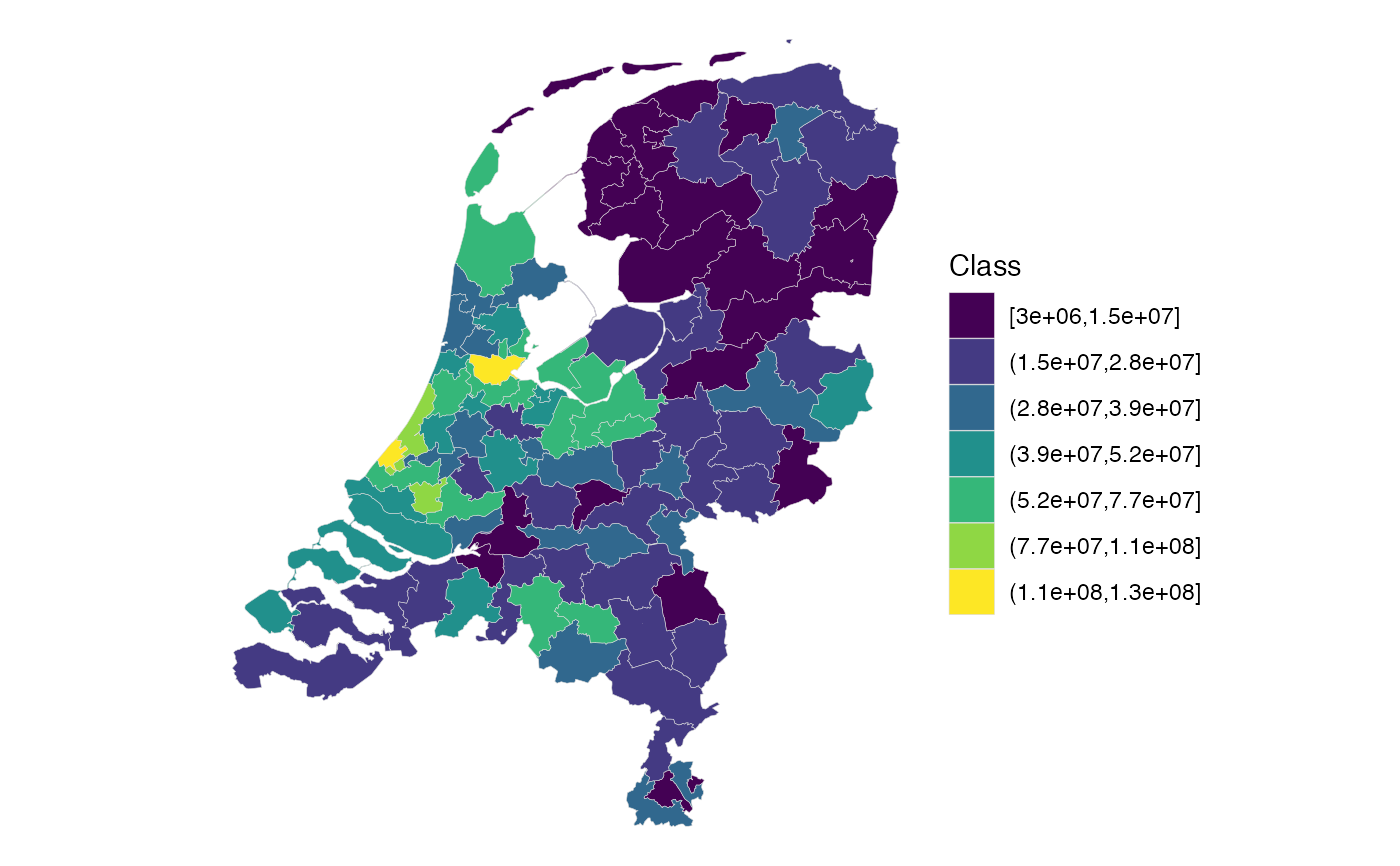
Creates a choropleth map from an object of class sf.
If the chosen variable can be classified into discrete intervals using
Fisher's natural breaks, the polygons are shaded by cluster. Otherwise,
the variable is visualized on a continuous scale.
Usage
choropleth_ggplot2(
  sf_object,
  value = output,
  n = 7,
  dig.lab = 2,
  legend_title = "Class",
  option = "D",
  direction = 1
)
Arguments
- sf_object
An object of class
sfcontaining polygon geometries.- value
Column in
sf_objectused to shade the polygons (default =output).- n
Integer. Number of clusters to use in Fisher classification (default = 7).
- dig.lab
Integer. Number of digits to display in legend labels (default = 2).
- legend_title
Character. Title for the legend (default = "Class").
- option
Character string indicating the colormap option passed to
viridis. Options are:"magma"(or"A")"inferno"(or"B")"plasma"(or"C")"viridis"(or"D", default)"cividis"(or"E")
- direction
Numeric. Order of colors in the scale. If
1(default), colors go from darkest to lightest. If-1, the order is reversed.
Details
The function first attempts to classify the chosen variable into
n clusters using Fisher's natural breaks
(classInt::classIntervals()). If this fails (e.g. due to insufficient
unique values), the function falls back to a continuous scale.
Examples
test <- points_to_polygon(
  nl_postcode2,
  insurance,
  sum(amount, na.rm = TRUE)
)
#> 80 points are outside any polygon.
choropleth_ggplot2(test, value = output)

