spatialrisk is specifically designed for efficient spatial risk calculations, allowing users to quickly sum all observations within a defined radius. With key functions implemented in C++ using Rcpp, the package ensures fast performance for various spatial analysis tasks, including optimizing location and resource allocation.
Installation
Install spatialrisk from CRAN:
install.packages("spatialrisk")Or the development version from GitHub:
# install.packages("remotes")
remotes::install_github("MHaringa/spatialrisk")
Example 1: Observations Within a Defined Radius
Filter all observations in Groningen located within a 100-meter radius circle centered at coordinates (longitude, latitude) = (6.561561, 53.21326):
library(spatialrisk)
circle <- points_in_circle(Groningen, lon_center = 6.571561,
                           lat_center = 53.21326, radius = 100)
circle
## # A tibble: 14 × 10
## street number letter suffix postal_code city lon lat amount distance_m
## <chr> <int> <chr> <chr> <chr> <chr> <dbl> <dbl> <dbl> <dbl>
## 1 Heresin… 5 <NA> <NA> 9711EP Gron… 6.57 53.2 5 31.4
## 2 Heresin… 11 <NA> <NA> 9711ER Gron… 6.57 53.2 11 47.8
## 3 Zuiderp… 1003 <NA> <NA> 9724AK Gron… 6.57 53.2 1003 57.6
## 4 Heresin… 13 <NA> <NA> 9711ER Gron… 6.57 53.2 13 68.1
## 5 Hereple… 10 <NA> <NA> 9711GA Gron… 6.57 53.2 10 74.6
## 6 Heresin… 16 <NA> <NA> 9711ES Gron… 6.57 53.2 16 84.1
## 7 Heresin… 6 <NA> <NA> 9711ES Gron… 6.57 53.2 6 86.2
## 8 Heresin… 6 a <NA> 9711ES Gron… 6.57 53.2 6 87.8
## 9 Heresin… 6 b <NA> 9711ES Gron… 6.57 53.2 6 90.9
## 10 Heresin… 20 <NA> <NA> 9711ET Gron… 6.57 53.2 20 91.5
## 11 Heresin… 20 a <NA> 9711ET Gron… 6.57 53.2 20 93.0
## 12 Heresin… 15 a <NA> 9711ER Gron… 6.57 53.2 15 95.1
## 13 Zuiderp… 1007 <NA> <NA> 9724AK Gron… 6.57 53.2 1007 97.2
## 14 Zuiderp… 25 a <NA> 9724AJ Gron… 6.57 53.2 25 97.8The sum of all observations within this circle is equal to:
sum(circle$amount)Next, calculate the sum of all observations within a specified radius. concentration() computes the total sum of all observations within a circle of a given radius for multiple locations. For each row in df, it finds the sum of all observations in Groningen that fall within a 100-meter radius from the specified (lon, lat) coordinates.
df <- data.frame(location = c("p1", "p2", "p3"),
                 lon = c(6.561561, 6.561398, 6.571561),
                 lat = c(53.21369, 53.21326, 53.21326))

conc <- concentration(df, Groningen, value = amount, radius = 100)
conc
## location lon lat concentration
## 1 p1 6.561561 53.21369 775
## 2 p2 6.561398 53.21326 2271
## 3 p3 6.571561 53.21326 2163Show that result is indeed equal to the result from the previous example:
Example 2: Find Highest Concentrations
spatialrisk offers a fast and effective way to identify areas with the highest concentration of fire risks within a 200-meter radius—meeting a key requirement of the European Directive 2009/138 (Solvency II) and aligned with the principles of the Maximal Covering Location Problem (MCLP). While the directive doesn’t mandate a specific method, spatialrisk provides a clear and systematic approach to mapping high-risk clusters. This helps insurers accurately assess their maximum exposure to catastrophic fire events and adjust their solvency capital requirements in line with Solvency II standards.
Under Solvency II, the fire risk challenge involves calculating the capital requirement for fire-related events—such as fires, explosions, and terrorist attacks—by identifying the largest concentration of insured assets at risk. This can be approached as a location optimization problem: finding the optimal center of a fixed-radius circle that captures the maximum total value of insured fire risks within that area. The structure of this problem closely mirrors the Maximal Covering Location Problem (MCLP), a well-established model in operations research used to maximize coverage within a limited range.
The Maximal Covering Location Problem (MCLP)
Originally proposed by Church and ReVelle in 1974, the Maximal Covering Location Problem (MCLP) focuses on placing facilities in locations that maximize coverage of demand points within a predefined distance. In this context:
- Demand points represent locations that require coverage, such as populations, assets, or infrastructure.
- Facilities are placed to cover as many of these points as possible, within a fixed coverage radius.
- The goal is to maximize total demand covered using a limited number of facilities and a set coverage distance.
Strategic Rationale for Applying MCLP to Fire Risk Assessment
The Solvency II directive requires insurers to assess their capital exposure to fire risk by identifying the highest concentration of insured assets within a 200-meter radius. This challenge aligns closely with the Maximal Covering Location Problem (MCLP), a proven model from operations research used to optimize coverage within a fixed area. The similarities are clear:
- Valuable Assets as Demand Points: Each insured building or asset is treated as a demand point, similar to how MCLP models locations needing coverage.
- Fixed 200-Meter Radius: The regulatory requirement mirrors MCLP’s coverage radius—assets are either within range or not.
- Focus on Maximum Exposure: Just as MCLP aims to maximize covered demand, the fire risk assessment seeks to identify the location with the greatest insured value concentration.
Algorithm: Maximal Covering Location Problem (MCLP) via Raster Analysis
Overview
This algorithm presents a practical and scalable solution for identifying high-risk locations using the Maximal Covering Location Problem (MCLP), implemented through spatial raster analysis. Built on the robust capabilities of the terra package in R, the approach transforms complex spatial data into actionable insights. It enables insurers and urban planners to pinpoint areas of highest risk concentration.
Key Steps in the Process
1. Aggregating Spatial Risk Data
Objective: Create a simplified, high-level view of demand concentrations.
- Spatial data points (e.g., insured assets) are converted into a raster grid with 50 x 50 meter cells.
- Each cell summarizes the total insured value within its boundaries, creating a spatial heatmap of risk exposure.
2. Highlighting High-Risk Clusters
Objective: Identify areas where demand values cluster within proximity.
- Using focal statistics, the algorithm analyzes each cell and its neighbors to highlight broader risk concentrations.
- A weighting matrix refines this analysis, revealing where the most significant clusters lie.
3. Focusing the Search
Objective: Narrow in on the top risk zones.
- The algorithm selects the top five areas with the highest aggregated risk values.
- Within each, it builds a detailed 20 x 20 grid (400 sub-points) to begin exploring optimal facility or response locations.
4. Refining to High-Potential Zones
Objective: Eliminate low-impact areas and zoom in on promising locations.
- Only zones that exceed a calculated risk threshold (lower bound) are retained.
- These areas are then mapped at a finer 1-meter resolution, concentrating analysis where it matters most.
5. Pinpointing Optimal Locations
Objective: Identify the exact spots offering maximum coverage potential.
- A high-resolution grid is generated within the selected areas.
- The algorithm evaluates each point’s ability to cover surrounding demand, producing a shortlist of optimal locations for intervention, resource allocation, or risk management.
Illustrative Example: Identifying Areas of Highest Risk Concentration
As a practical application of the above methodology, this example demonstrates how the algorithm can calculate the total demand (e.g., insured value) within a fixed radius around multiple locations.
find_highest_concentration() is used to determine the central coordinates of a circle with a constant radius that captures the maximum sum of surrounding demand points. This enables decision-makers—such as insurers or urban planners—to pinpoint where risk is most densely concentrated and where targeted action can yield the greatest impact.
In this case, the method is applied to the Groningen dataset, which contains spatial risk points relevant to the analysis.
Visualization:
Display all spatial demand points from the Groningen dataset as a foundation for identifying optimal coverage locations.
plot_points(Groningen, value = "amount")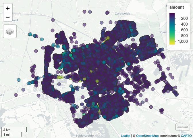
Determine the Optimal Central Location for Maximum Risk Coverage:
In this step, the goal is to determine the central coordinates of a circular area that captures the highest concentration of demand. Using a fixed radius, the algorithm systematically scans all potential locations, calculating the total risk value within each surrounding area.
To support fast and scalable analysis, all core functions are written in C++. This ensures high-performance computation, allowing the algorithm to handle large and complex spatial datasets with exceptional speed and efficiency.
By applying find_highest_concentration(), we isolate the point that offers the greatest cumulative coverage:
hc <- find_highest_concentration(Groningen,
                                 value = "amount",
                                 radius = 200)
hc[[1]]Visualizing the Area of Highest Concentration:
Plot the individual points located within the highest concentration zone. The total sum of their values corresponds to the reported concentration figure.
This area represents the highest demand concentration in the Groningen dataset. It notably includes two apartment buildings containing a large number of insured objects, which significantly contribute to the overall risk exposure.
plot(hc)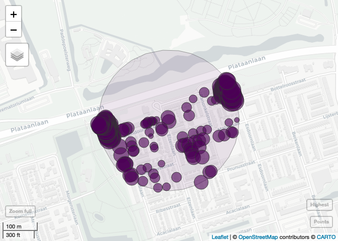
It is also possible to display the coordinates for multiple high-concentration areas. To visualize the second and third highest concentrations:
hconc <- find_highest_concentration(Groningen,
                                    value = "amount",
                                    radius = 200,
top_n = 3)Create interactive map:
plot(hconc)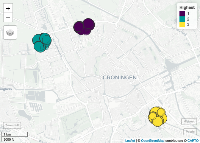
Display the objects located within the highest concentration circle:
hc[[2]]## # A tibble: 208 × 13
## street number letter suffix postal_code city lon lat amount ix
## <chr> <int> <chr> <chr> <chr> <chr> <dbl> <dbl> <dbl> <int>
## 1 Elzenlaan 135 <NA> <NA> 9741ND Gron… 6.55 53.2 135 20449
## 2 Elzenlaan 139 <NA> <NA> 9741ND Gron… 6.55 53.2 139 23229
## 3 Elzenlaan 70 <NA> <NA> 9741NG Gron… 6.55 53.2 70 585
## 4 Elzenlaan 68 <NA> <NA> 9741NG Gron… 6.55 53.2 68 14677
## 5 Duindoornstr… 1 <NA> <NA> 9741NM Gron… 6.55 53.2 12 16828
## 6 Duindoornstr… 17 <NA> <NA> 9741NM Gron… 6.55 53.2 17 12829
## 7 Duindoornstr… 15 <NA> <NA> 9741NM Gron… 6.55 53.2 15 16004
## 8 Duindoornstr… 21 <NA> <NA> 9741NM Gron… 6.55 53.2 21 11748
## 9 Duindoornstr… 13 <NA> <NA> 9741NM Gron… 6.55 53.2 13 2006
## 10 Ranonkelstra… 38 <NA> <NA> 9741LT Gron… 6.55 53.2 38 19696
## # ℹ 198 more rows
## # ℹ 3 more variables: distance_m <dbl>, id <int>, conc <dbl>Example 3: Creating Choropleth Maps
spatialrisk also offers features for creating choropleth maps, which can be challenging in R. points_to_polygon() provides an elegant solution to this issue.
Typically, creating choropleths involves aggregating data at the regional level of the shapefile and then merging this aggregated data with the shapefile. However, this method can be problematic if the names in the data do not match those in the shapefile, such as when there are differences in punctuation or spelling in area names. To address this, points_to_polygon() uses the longitude and latitude of a point to accurately map it to the corresponding region. This approach simplifies the creation of choropleth maps at various regional levels.
For example, points_to_polygon() can be used to visualize the total sum insured at the municipality level across the Netherlands:
gemeente_sf <- points_to_polygon(nl_gemeente, insurance, sum(amount, na.rm = TRUE))choropleth() generates a map from the simple feature object created in the previous step. There are two ways to create a choropleth map: if you set the mode to plot, it produces a static map. The clustering in this case is based on the Fisher-Jenks algorithm, a widely used method for classifying data in choropleth maps.
choropleth(gemeente_sf, mode = "plot", legend_title = "Sum insured (EUR)", n = 5)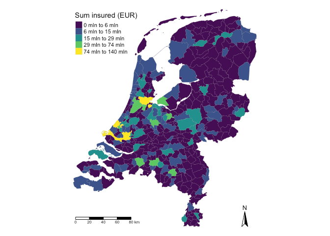
If mode is set to view an interactive map is created:
choropleth(gemeente_sf, mode = "view", legend_title = "Sum insured (EUR)")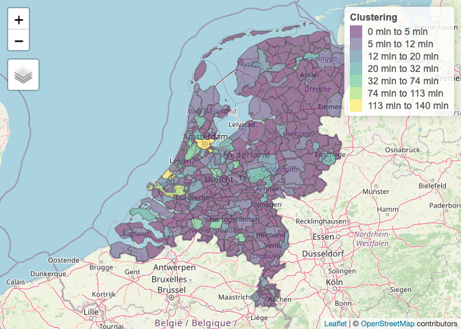
The following simple feature objects are available in spatialrisk: nl_provincie, nl_corop, nl_gemeente, nl_postcode1, nl_postcode2, nl_postcode3, nl_postcode4, world_countries, and europe_countries.
