Getting started

Introduction

insurancerating provides actuarial building blocks for insurance pricing in R.

A common GLM-based pricing exercise often combines several tasks:

1. portfolio analysis
2. model estimation
3. interpretation of fitted coefficients
4. refinement of tariff structure

This vignette illustrates one way to combine the main building blocks:

• analyse risk factors with factor_analysis()
• estimate pricing models with glm()
• interpret coefficients with rating_table()
• assess model stability with model_performance() and bootstrap_performance()

The focus is on the transition from portfolio data to an interpretable tariff structure.

Data

We use the example dataset MTPL2, which contains a motor portfolio with:

• number of claims (nclaims),
• exposure (exposure),
• premium (premium),
• claim amounts (amount),
• several rating factors

library(insurancerating)
library(dplyr)

head(MTPL2)
#> # A tibble: 6 × 6
#>   customer_id  area nclaims amount exposure premium
#>         <int> <int>   <int>  <int>    <dbl>   <int>
#> 1       92617     2       0      0   1           90
#> 2      120632     2       0      0   1           82
#> 3      147800     2       0      0   1           47
#> 4       29763     3       0      0   0.0630      44
#> 5       61107     1       1   6066   1           69
#> 6        4318     3       0      0   1           66

Step 1 — Portfolio analysis

Factor analysis

A pricing analysis often starts with an analysis of the portfolio.

Before fitting a model, it is necessary to understand:

• how experience differs across factor levels
• whether differences are credible
• whether exposure is sufficient
• whether the observed pattern is plausible

This is done with factor_analysis().

Basic factor analysis

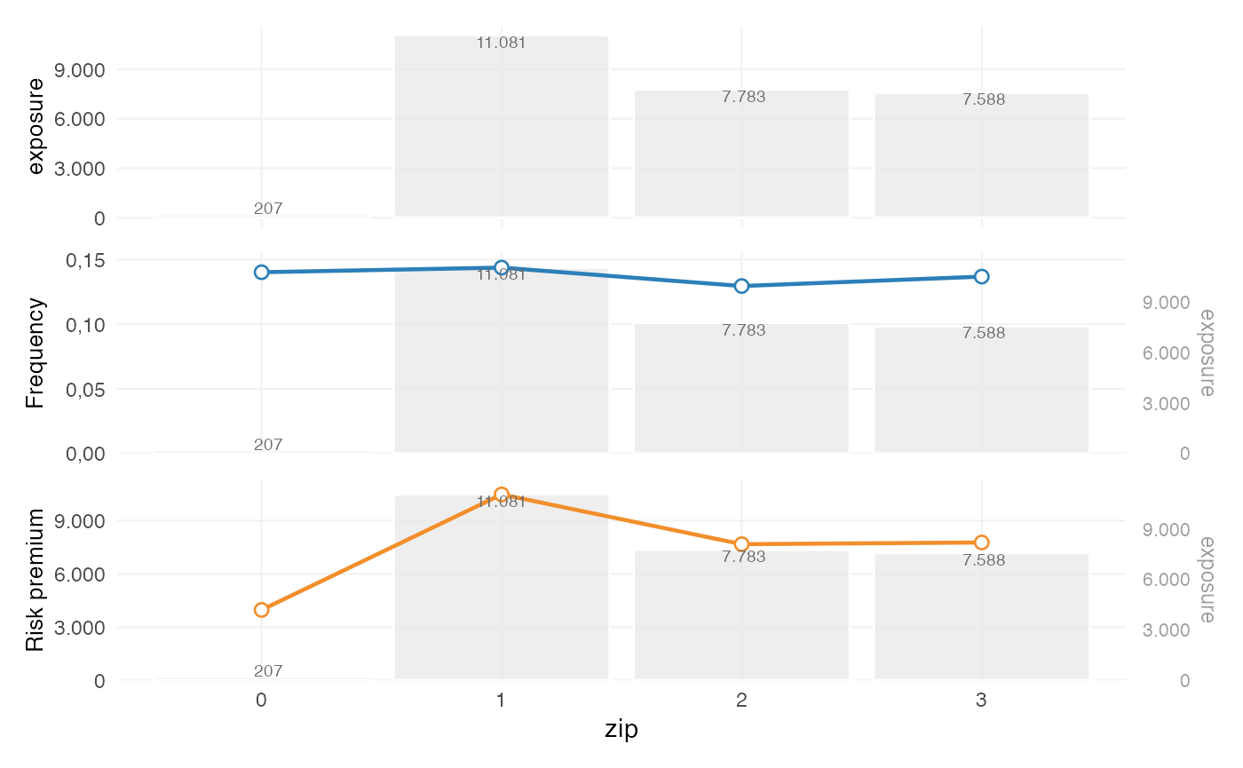
We start by analysing a single risk factor.

fa <- factor_analysis(
  MTPL,
  risk_factors = "zip",
  claim_count = "nclaims",
  exposure = "exposure",
  claim_amount = "amount"
)

fa
#>   zip    amount nclaims   exposure frequency average_severity risk_premium
#> 1   1 116178669    1593 11080.6274 0.1437644         72930.74    10484.846
#> 2   2  59751985    1008  7782.6301 0.1295192         59277.76     7677.608
#> 3   3  58988962    1038  7587.5644 0.1368028         56829.44     7774.427
#> 4   0    821510      29   206.8438 0.1402024         28327.93     3971.644

The output provides commonly used portfolio metrics such as:

• frequency = claims / exposure
• average severity = loss / claims
• risk premium = loss / exposure
• loss ratio = loss / premium
• average premium = premium / exposure

Visualising factor behaviour

autoplot(fa, metrics = c(6, 1, 3))

This provides a direct view of:

• the distribution of exposure
• the variation in claim frequency
• the variation in risk premium

At this stage, the purpose is not yet to fit a model, but to understand whether the factor behaves in a way that is suitable for pricing.

Step 2 — Continuous variables

Why continuous variables are treated separately

Continuous variables are typically not used directly in a tariff. In pricing practice, they are usually:

1. analysed as continuous variables
2. translated into tariff classes
3. used in a GLM as categorical rating factors

This ensures that the final tariff remains interpretable and implementable.

Analysing the shape with a GAM

age_freq <- risk_factor_gam(
  data = MTPL,
  risk_factor = "age_policyholder",
  claim_count = "nclaims",
  exposure = "exposure"
)

autoplot(age_freq, show_observations = TRUE)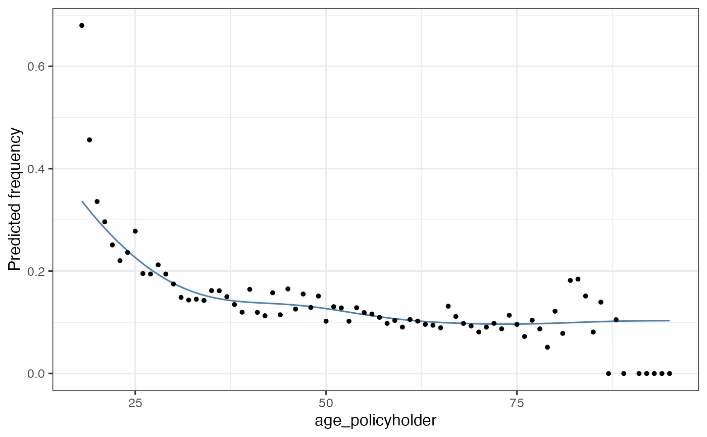

This step is used to inspect:

• non-linear patterns
• local volatility
• areas with low exposure
• plausible breakpoints for tariff classes

Constructing tariff classes

clusters <- construct_tariff_classes(age_freq)
autoplot(clusters)

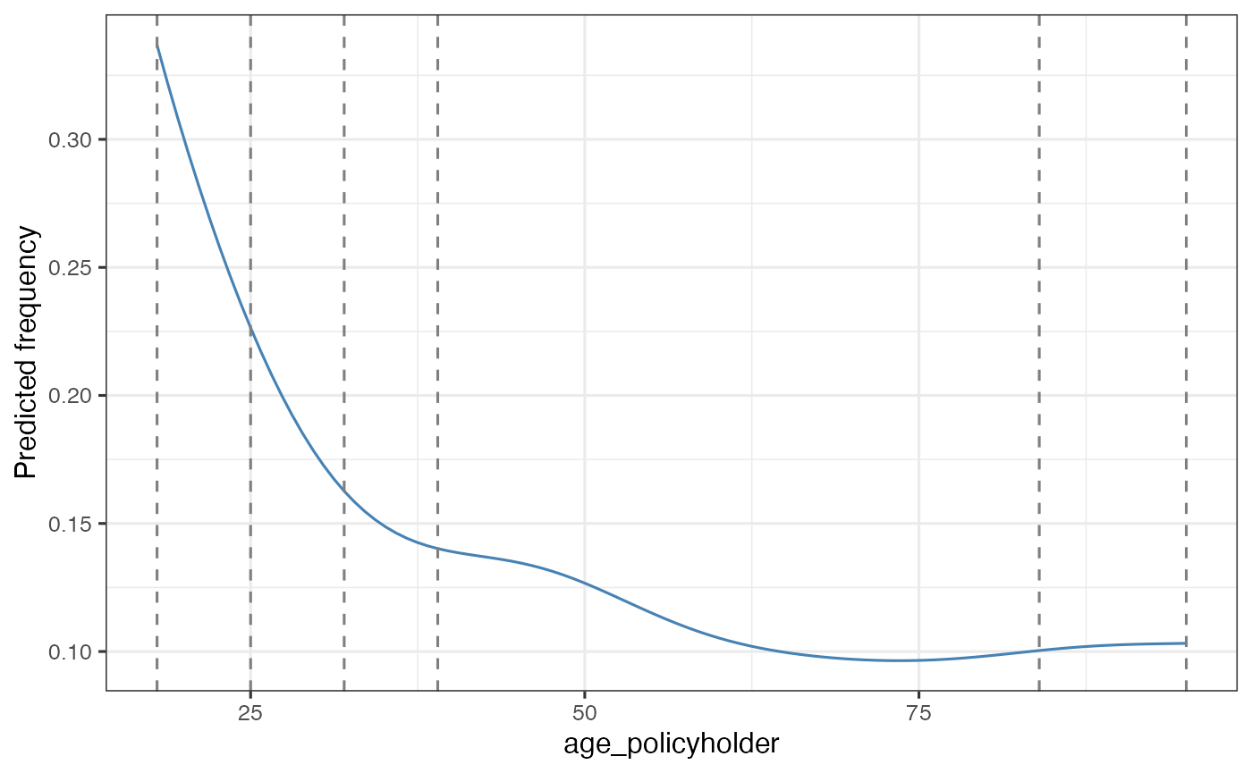
This converts the continuous variable into risk-homogeneous classes.

The resulting classes should reflect differences in risk, while remaining suitable for use in a tariff.

Adding tariff classes to the data

dat <- MTPL |>
  mutate(age_cat = clusters$tariff_classes) |>
  mutate(across(where(is.character), as.factor)) |>
  mutate(across(where(is.factor), ~ biggest_reference(., exposure)))

biggest_reference() sets the reference level to the level with the highest exposure. In pricing models, this is often the most stable and interpretable baseline.

Step 3 — Model estimation

Why GLMs are used

Generalized linear models are widely used in insurance pricing because they:

• accommodate non-normal response distributions
• produce interpretable multiplicative effects
• can be translated into tariff relativities

A common decomposition is:

• frequency –> Poisson GLM
• severity –> Gamma GLM

Frequency model

mod_freq <- glm(
  nclaims ~ age_cat,
  offset = log(exposure),
  family = poisson(),
  data = dat
)

Severity model

mod_sev <- glm(
  amount ~ age_cat,
  weights = nclaims,
  family = Gamma(link = "log"),
  data = dat |> filter(amount > 0)
)

Frequency and severity are modelled separately because they capture different aspects of the loss process.

Constructing a premium proxy

premium_df <- dat |>
  add_prediction(mod_freq, mod_sev) |>
  mutate(premium = pred_nclaims_mod_freq * pred_amount_mod_sev)

head(premium_df)
#>   age_policyholder nclaims  exposure amount power bm zip age_cat
#> 1               70       0 1.0000000      0   106  5   1 (65,84]
#> 2               40       0 1.0000000      0    74  3   1 (39,51]
#> 3               78       0 1.0000000      0    65  8   2 (65,84]
#> 4               49       0 1.0000000      0    64 10   1 (39,51]
#> 5               59       0 1.0000000      0    29  1   3 (58,65]
#> 6               71       0 0.4547945      0    66  6   3 (65,84]
#>   pred_nclaims_mod_freq pred_amount_mod_sev  premium
#> 1            0.10100599            67736.95 6841.837
#> 2            0.13595893            72328.67 9833.729
#> 3            0.10100599            67736.95 6841.837
#> 4            0.13595893            72328.67 9833.729
#> 5            0.09746194            57782.98 5631.642
#> 6            0.04593697            67736.95 3111.630

This produces a pure premium estimate, i.e. expected loss per unit of exposure.

Step 4 — Premium model

Fitting a premium model

burn_unrestricted <- glm(
  premium ~ age_cat + zip,
  weights = exposure,
  family = Gamma(link = "log"),
  data = premium_df
)

This model combines the rating factors into a single premium structure.

In practice, this is often the model that is closest to the final tariff logic, because it reflects the premium level rather than only individual model components such as frequency or severity.

Step 5 — Interpreting coefficients

Rating table

rt <- rating_table(burn_unrestricted)
rt
#>          level risk_factor est_burn_unrestricted exposure
#> 1  (Intercept) (Intercept)          9370.4023322       NA
#> 2            0         zip             0.9946246      207
#> 3            1         zip             1.0000000    11081
#> 4            2         zip             1.0049888     7783
#> 5            3         zip             1.0028308     7588
#> 6      [18,25]     age_cat             2.3041459     1331
#> 7      (25,32]     age_cat             2.4813038     3649
#> 8      (32,39]     age_cat             0.9246871     4247
#> 9      (39,51]     age_cat             1.0000000     7421
#> 10     (51,58]     age_cat             0.5699965     3245
#> 11     (58,65]     age_cat             0.5798450     2791
#> 12     (65,84]     age_cat             0.7103948     3901
#> 13     (84,95]     age_cat             0.5190330       72

rating_table() expresses fitted coefficients in terms of the original factor levels, including the reference level.

This output is commonly used to inspect tariff relativities.

Visualising coefficients

rating_table(burn_unrestricted, 
             model_data = premium_df, 
             exposure = "exposure") |>
  autoplot()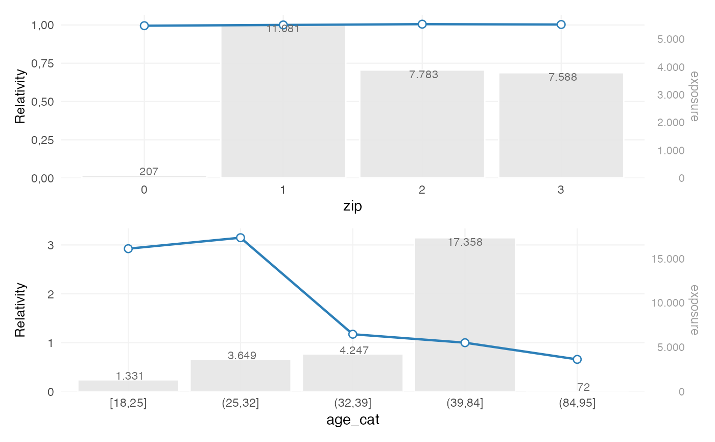

This plot is typically used to assess:

• the relative size of coefficients
• the structure across levels
• the exposure behind each level
• whether additional refinement may be needed

At this stage, the relevant questions are:

• are coefficients sufficiently stable?
• do they follow the expected pattern?
• are some levels driven by limited exposure?

Step 6 — Model evaluation

Model performance

model_performance(mod_freq)
#> # Comparison of Model Performance Indices
#> 
#>  Model   |   AIC    |    BIC    | RMSE  
#> ---------+----------+-----------+------ 
#> mod_freq | 22949.04 | 23015.512 | 0.362

This provides summary measures of model fit, such as RMSE.

Bootstrap performance

bp <- bootstrap_performance(mod_freq, dat, n_resamples = 50, show_progress = FALSE)
autoplot(bp)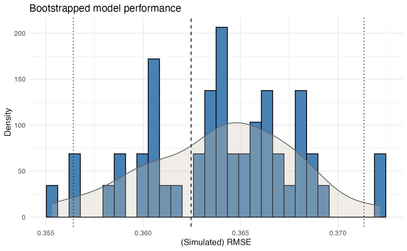

This provides a view of predictive stability by evaluating how performance changes across bootstrap samples.

A single fit statistic is usually not sufficient. In pricing practice, it is also relevant to assess whether the model behaves consistently under small data perturbations.

Step 7 — From model to tariff

At this point, the example has produced:

• portfolio-level insight
• fitted pricing models
• interpretable factor relativities
• basic performance diagnostics

In many cases, a further step is required before the model output can be used as a tariff.

Typical reasons include:

• irregular coefficient patterns
• monotonicity requirements
• externally imposed restrictions
• expert-driven adjustments

This can be handled with the refinement tools described in Refinement building blocks.

Summary

A possible sequence in insurancerating is:

factor_analysis()             # analyse portfolio behaviour
risk_factor_gam()              # analyse continuous variables
construct_tariff_classes()    # derive tariff classes
glm()                         # estimate pricing models
rating_table()                # interpret fitted coefficients
bootstrap_performance()       # assess stability
prepare_refinement()          # refine tariff structure if needed

The aim is to move from raw portfolio data to a tariff structure that is:

• interpretable
• reproducible
• and suitable for practical pricing use

Next steps

The following vignette covers the refinement step in more detail:

• Refinement building blocks

For the conceptual background to exposure, risk premium, and tariff design, see:

• Pricing principles