Pricing workflow building blocks • insurancerating

insurancerating provides building blocks for common actuarial pricing tasks in GLM-based tariff analysis. The package does not prescribe a single pricing method. Instead, it supports practical steps that often appear in insurance pricing work: portfolio analysis, model interpretation, tariff refinement and model validation.

This vignette gives a compact overview of those building blocks and how they can be combined.

library(insurancerating)

1. Start with portfolio experience

A pricing analysis often starts by checking how the observed portfolio behaves by risk factor. This is useful before modelling, but also later when reviewing whether fitted relativities are plausible.

factor_analysis() summarises exposure, claim frequency, average severity, risk premium and related metrics by one or more risk factors.

fa <- factor_analysis(
  MTPL,
  risk_factors = "zip",
  claim_count = "nclaims",
  claim_amount = "amount",
  exposure = "exposure"
)

head(fa)
#>   zip    amount nclaims   exposure frequency average_severity risk_premium
#> 1   1 116178669    1593 11080.6274 0.1437644         72930.74    10484.846
#> 2   2  59751985    1008  7782.6301 0.1295192         59277.76     7677.608
#> 3   3  58988962    1038  7587.5644 0.1368028         56829.44     7774.427
#> 4   0    821510      29   206.8438 0.1402024         28327.93     3971.644

The output helps answer practical questions such as:

where exposure is concentrated
whether observed differences are credible or noisy
whether a segment is driven by a small number of claims
which risk factors may need closer modelling or refinement

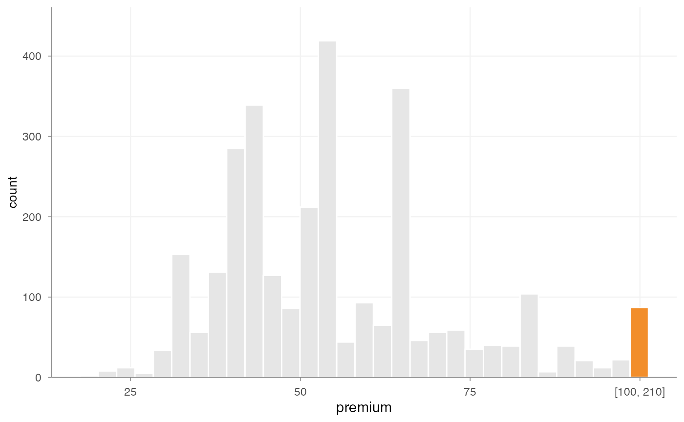
For numeric variables with long or skewed tails, outlier_histogram() can help inspect extreme observations before fitting severity models or constructing tariff segments.

outlier_histogram(
  MTPL2,
  x = "premium",
  upper = 100,
  density = FALSE
)

2. Assess large losses

Large claims can dominate severity and pure premium analysis. In capped severity workflows, it is often useful to assess a cap first, decompose the historical claim amounts, and then decide how the excess burden should be allocated. A low threshold increases pricing responsiveness but introduces volatility. A high threshold improves stability but may understate structural differences between segments.

thresholds <- assess_excess_threshold(
  claims,
  claim_amount = "claim_amount",
  thresholds = c(50000, 100000, 150000),
  exposure = "earned_exposure",
  group = "sector"
)

autoplot(thresholds, y = "premium_impact")

After choosing a threshold, calculate_excess_loss() creates a deterministic historical decomposition. It does not bootstrap or allocate anything.

excess <- calculate_excess_loss(
  claims,
  claim_amount = "claim_amount",
  threshold = 100000
)

The allocation step is where pooling and uncertainty are handled. Portfolio pooling is stable but ignores group experience. Group pooling is responsive but can be volatile. Partial pooling balances portfolio stability, group responsiveness and the credibility of observed excess experience.

allocation <- allocate_excess_loss(
  excess,
  excess_amount = "excess_claim_amount",
  weight = "earned_exposure",
  group = "sector",
  pooling = "partial",
  preserve_total = TRUE
)

summary(allocation, compare_to_empirical = TRUE)
autoplot(allocation, y = "allocated_loading")
autoplot(allocation, y = "credibility")

In the allocation output, allocated_excess_loss is the absolute monetary burden assigned to a row. allocated_loading is the corresponding loading per unit of the chosen weight, such as earned exposure. This distinction matters when the output is added back to pricing data.

The allocated loading can then be added to the pricing data.

excess$base_premium <- excess$technical_premium
priced <- add_excess_loading(
  excess,
  allocation,
  base_premium = "base_premium"
)

This excess loading is part of the technical risk premium. It is not intended as a commercial margin.

3. Translate continuous factors into tariff segments

Many tariffs use grouped versions of continuous variables such as age, vehicle age or insured value. risk_factor_gam() can be used to inspect the fitted shape of a continuous risk factor. derive_tariff_segments() can then derive candidate segment boundaries from that pattern.

age_gam <- risk_factor_gam(
  data = MTPL,
  claim_count = "nclaims",
  risk_factor = "age_policyholder",
  exposure = "exposure"
)

age_segments <- derive_tariff_segments(age_gam)
age_segments
#> Tariff segment boundaries:
#> [1] 18 25 32 39 51 58 65 84 95

The derived segments can be added back to the portfolio with add_tariff_segments().

portfolio <- MTPL |>
  add_tariff_segments(age_segments, name = "age_policyholder_segment")

head(portfolio[, c("age_policyholder", "age_policyholder_segment")])
#> # A tibble: 6 × 2
#>   age_policyholder age_policyholder_segment
#>              <int> <fct>                   
#> 1               70 (65,84]                 
#> 2               40 (39,51]                 
#> 3               78 (65,84]                 
#> 4               49 (39,51]                 
#> 5               59 (58,65]                 
#> 6               71 (65,84]

These functions are intended to support actuarial judgement, not replace it. Candidate segment boundaries should still be reviewed for credibility, stability and practical usability.

4. Fit and interpret a GLM

GLMs are widely used in insurance pricing because they provide an interpretable multiplicative structure. After fitting a model, rating_table() expresses the coefficients in tariff-table form.

portfolio$zip <- as.factor(portfolio$zip)

freq_model <- glm(
  nclaims ~ zip + age_policyholder_segment + offset(log(exposure)),
  family = poisson(),
  data = portfolio
)

rt <- rating_table(
  freq_model,
  model_data = portfolio,
  exposure = "exposure"
)

head(rt$df)
#>                risk_factor       level est_freq_model exposure
#> 1              (Intercept) (Intercept)      0.2743790       NA
#> 2                      zip           0      1.0000000      207
#> 3                      zip           1      0.9944341    11081
#> 4                      zip           2      0.8960053     7783
#> 5                      zip           3      0.9493475     7588
#> 6 age_policyholder_segment     [18,25]      1.0000000     1331

Observed portfolio experience from factor_analysis() can be attached to the rating table with add_observed_experience(). This makes the comparison between model relativities and observed experience explicit.

zip_experience <- factor_analysis(
  portfolio,
  risk_factors = "zip",
  claim_count = "nclaims",
  exposure = "exposure"
)

rt |>
  add_observed_experience(zip_experience, metric = "frequency") |>
  autoplot(risk_factors = "zip")

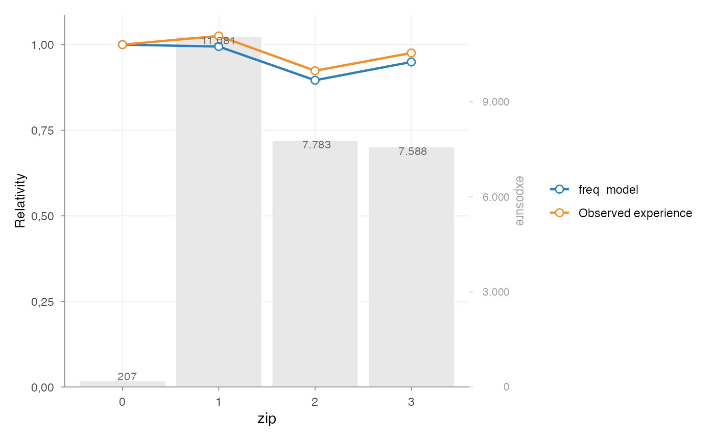
5. Refine tariff effects when needed

Raw model output may be statistically valid but still unsuitable for direct tariff use. Sparse levels, noisy estimates or non-monotonic adjacent effects can make a tariff hard to explain or maintain.

The refinement workflow makes these adjustments explicit:

refined_model <- prepare_refinement(freq_model) |>
  add_smoothing(
    model_variable = "age_policyholder_segment",
    source_variable = "age_policyholder",
    weights = "exposure"
  ) |>
  add_restriction(restrictions) |>
  refit()

Common refinement tasks include:

smoothing adjacent tariff levels
fixing selected coefficients to actuarial or commercial assumptions
applying sublevel relativities within a broader GLM factor level
refitting the model while preserving the intended tariff structure

These tools are most useful when the statistical model already captures the main risk structure and the remaining work is tariff refinement.

6. Validate model behaviour

Pricing models should be checked before their output is used in a tariff. insurancerating contains helpers for several common checks:

check_overdispersion() for Poisson frequency models
check_residuals() for simulation-based residual diagnostics using DHARMa
bootstrap_performance() for predictive stability with metrics such as RMSE
rating_grid() to inspect observed rating-grid combinations

For example:

check_overdispersion(freq_model)
#> Dispersion ratio =     1.185
#> Pearson's Chi-squared = 35522.367
#> p-value =   < 0.001
#> Overdispersion detected.

check_residuals(freq_model) |>
  autoplot()

Validation does not make a tariff decision by itself. It gives evidence about model fit, stability and areas that may need further review.

Typical workflow

One possible workflow is:

Inspect the portfolio with factor_analysis() and outlier_histogram().
Assess large-loss thresholds with assess_excess_threshold() where capped severity or excess-loss loadings are relevant.
Decompose and allocate excess loss with calculate_excess_loss() and allocate_excess_loss().
Analyse continuous risk factors with risk_factor_gam().
Create candidate tariff segments with derive_tariff_segments().
Fit GLMs for frequency, severity or pure premium.
Interpret coefficients with rating_table().
Compare fitted relativities with observed experience using add_observed_experience().
Apply refinement where needed with prepare_refinement(), add_smoothing(), add_restriction() or add_relativities().
Validate the resulting model with the model-performance helpers.

The exact order and choice of functions depends on the portfolio, product, data quality and pricing objective.

Next steps

For a worked example, see:

Getting started

For coefficient refinement:

Refinement building blocks

For validation:

Model validation