Refinement workflow

Introduction

In insurance pricing, model estimation is usually not the final step.

A fitted GLM may capture the structure of the portfolio well, but the raw coefficients are not always directly suitable for implementation in a tariff.

Common reasons include:

irregular local variation
lack of monotonicity
externally imposed tariff structures
expert judgement not directly represented in the model
implementation constraints in policy administration systems

For this reason, pricing workflows typically distinguish between:

model estimation
tariff refinement
final refit of the pricing structure

insurancerating formalises this through a staged refinement workflow:

fit an unrestricted model
initialise a refinement object with prepare_refinement()
add one or more refinement steps
inspect these steps before refit
call refit() to obtain the final fitted model

This separation makes the workflow easier to understand, reproduce, and audit.

Refinement is used when the estimated model output is statistically acceptable, but not yet suitable as a tariff structure.

Typical use cases include:

smoothing a rating factor derived from a continuous variable
imposing monotonicity
restricting coefficients to a predefined relativity structure
introducing expert-based relativities within existing model levels
simplifying the final tariff for practical implementation

In most cases, refinement is applied to the premium model, rather than to the separate frequency or severity models. The purpose of refinement is not primarily to smooth intermediate model components, but to impose structure on the final pricing signal that will be used in the tariff.

Example setup

The workflow below starts from a standard premium modelling setup:

analyse a continuous variable with a GAM
convert it to tariff classes
fit frequency and severity models
combine both into a premium proxy
fit an unrestricted premium model


library(insurancerating)
library(dplyr)

age_policyholder_frequency <- riskfactor_gam(
  data = MTPL,
  nclaims = "nclaims",
  x = "age_policyholder",
  exposure = "exposure"
)

clusters_freq <- construct_tariff_classes(age_policyholder_frequency)

dat <- MTPL |>
  mutate(age_policyholder_freq_cat = clusters_freq$tariff_classes) |>
  mutate(across(where(is.character), as.factor)) |>
  mutate(across(where(is.factor), ~ biggest_reference(., exposure)))

freq <- glm(
  nclaims ~ bm + age_policyholder_freq_cat,
  offset = log(exposure),
  family = poisson(),
  data = dat
)

sev <- glm(
  amount ~ zip,
  weights = nclaims,
  family = Gamma(link = "log"),
  data = dat |> filter(amount > 0)
)

premium_df <- dat |>
  add_prediction(freq, sev) |>
  mutate(premium = pred_nclaims_freq * pred_amount_sev)

burn_unrestricted <- glm(
  premium ~ zip + bm + age_policyholder_freq_cat,
  weights = exposure,
  family = Gamma(link = "log"),
  data = premium_df
)

Before refinement, inspect the unrestricted coefficient structure:


rating_table(burn_unrestricted)
#>                  risk_factor       level est_burn_unrestricted
#> 1                (Intercept) (Intercept)          1.073720e+04
#> 2                        zip           1          1.000000e+00
#> 3                        zip           0          3.739250e-01
#> 4                        zip           2          7.575359e-01
#> 5                        zip           3          7.325754e-01
#> 6  age_policyholder_freq_cat     (39,84]          1.000000e+00
#> 7  age_policyholder_freq_cat     [18,25]          2.167946e+00
#> 8  age_policyholder_freq_cat     (25,32]          1.488489e+00
#> 9  age_policyholder_freq_cat     (32,39]          1.205259e+00
#> 10 age_policyholder_freq_cat     (84,95]          5.868964e-01
#> 11                        bm          bm          9.980489e-01

rating_table(burn_unrestricted, 
             model_data = premium_df, 
             exposure = "exposure") |>
  autoplot()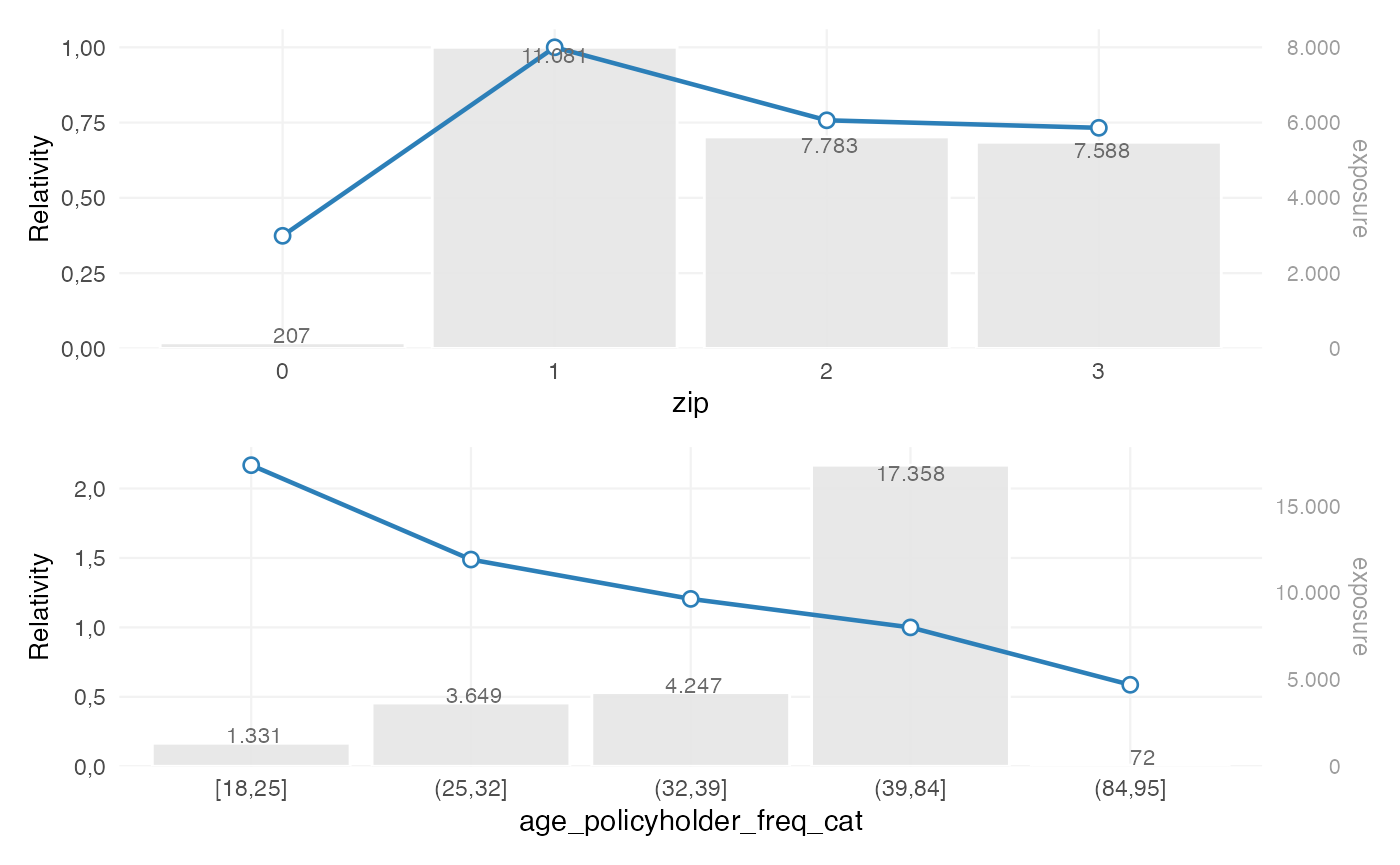

At this stage, the coefficients reflect the unrestricted model fit. In practice, this output may already be informative, but still too irregular or too detailed for direct tariff use.

Refinement begins with:


ref <- prepare_refinement(burn_unrestricted)
ref
#> <rating_refinement>
#> Base model: glm, lm
#> Steps: 0

A rating_refinement object stores:

the fitted base model
the underlying model data
the refinement steps added to the workflow

At this point, the model itself has not been refitted. The refinement object represents a proposed tariff adjustment structure, not yet the final fitted result.

This distinction is deliberate: refinement steps can be inspected before they are incorporated into the final model.

Smoothing

Purpose

Smoothing is used when a rating factor derived from a continuous variable contains undesirable local variation.

For example, a coefficient pattern such as:

age 30–34 lower
age 34–38 higher
age 38–42 lower again

may be statistically possible, but undesirable in a tariff. Smoothing imposes a more stable structure on the rating factor.

Adding smoothing


ref <- ref |>
  add_smoothing(
    x_cut = "age_policyholder_freq_cat",
    x_org = "age_policyholder",
    breaks = seq(18, 95, 5),
    weights = "exposure"
  )

The key arguments are:

x_cut: the binned factor present in the GLM
x_org: the original continuous variable
breaks: the preferred commercial cut points
smoothing: the smoothing specification
weights: optional weighting, typically exposure

Inspecting smoothing before refit


print(ref)
#> <rating_refinement>
#> Base model: glm, lm
#> Steps: 1
#> 1. smoothing [age_policyholder_freq_cat]
autoplot(ref, variable = "age_policyholder_freq_cat")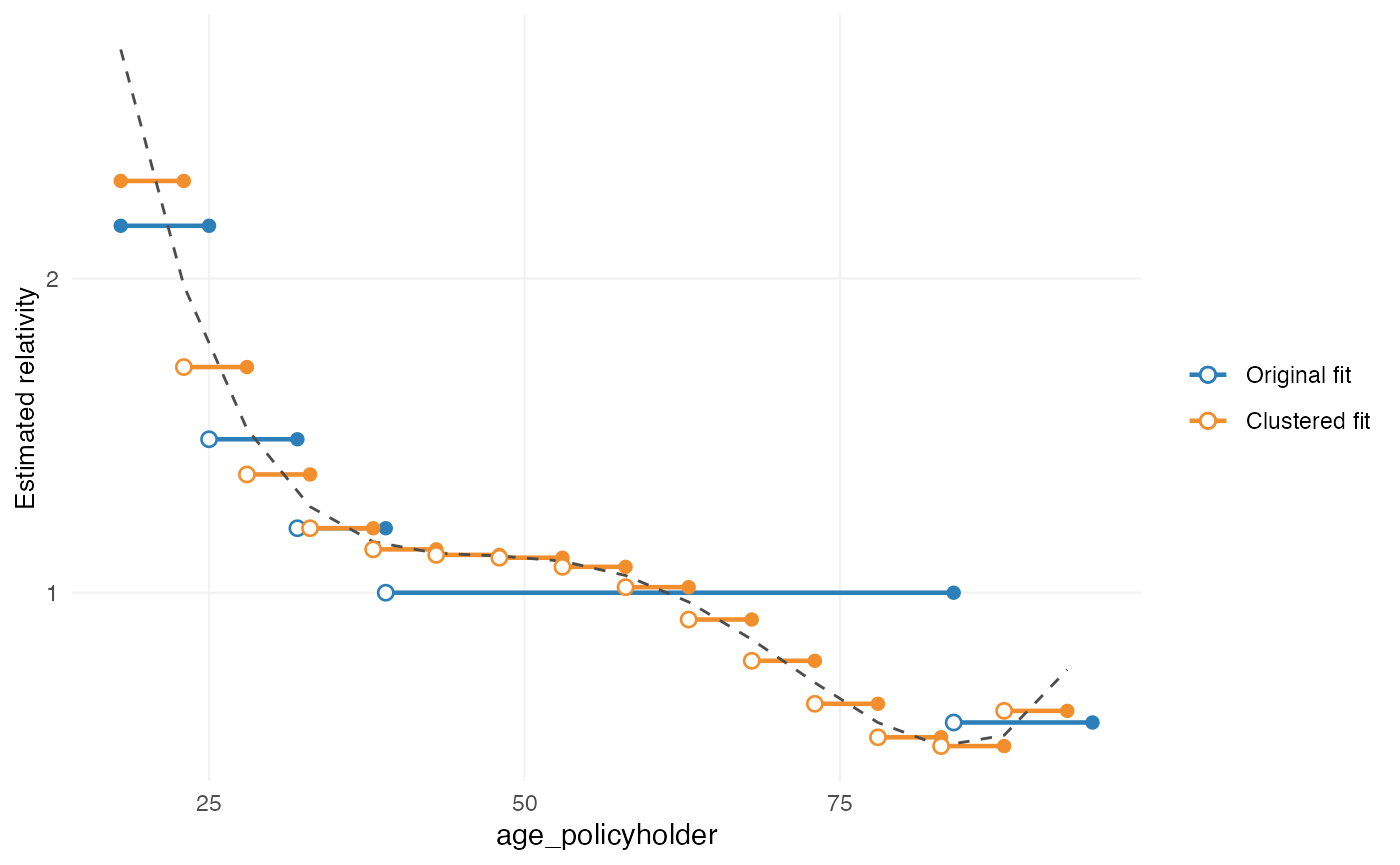

This plot belongs to the pre-refit workflow. It shows:

the original fitted coefficients
the proposed smoothed structure

The purpose is to inspect the refinement step itself, before it is incorporated into the final fitted model.

Choosing a smoothing method

Typical smoothing choices are:

"spline": polynomial-style smoothing
"gam": flexible smooth curve
"mpi": monotone increasing
"mpd": monotone decreasing

The appropriate choice depends on the pricing context.

For example:

age may justify a flexible smooth
insured value or power may require a monotonic relationship
low-exposure tails may benefit from exposure weighting

Restrictions

Purpose

Restrictions are used when coefficients must follow a predefined structure.

Typical examples include:

bonus-malus systems
governance-approved relativities
externally mandated tariff structures
implementation constraints in policy systems

Restrictions differ from smoothing:

smoothing reshapes the fitted pattern
restriction imposes user-defined coefficients

Adding restrictions


zip_df <- data.frame(
  zip = c(0, 1, 2, 3),
  zip_adj = c(0.8, 0.9, 1.0, 1.2)
)

ref <- ref |>
  add_restriction(restrictions = zip_df)

The restriction table must contain exactly two columns:

the original factor levels
the adjusted coefficients

Inspecting restrictions before refit


autoplot(ref, variable = "zip")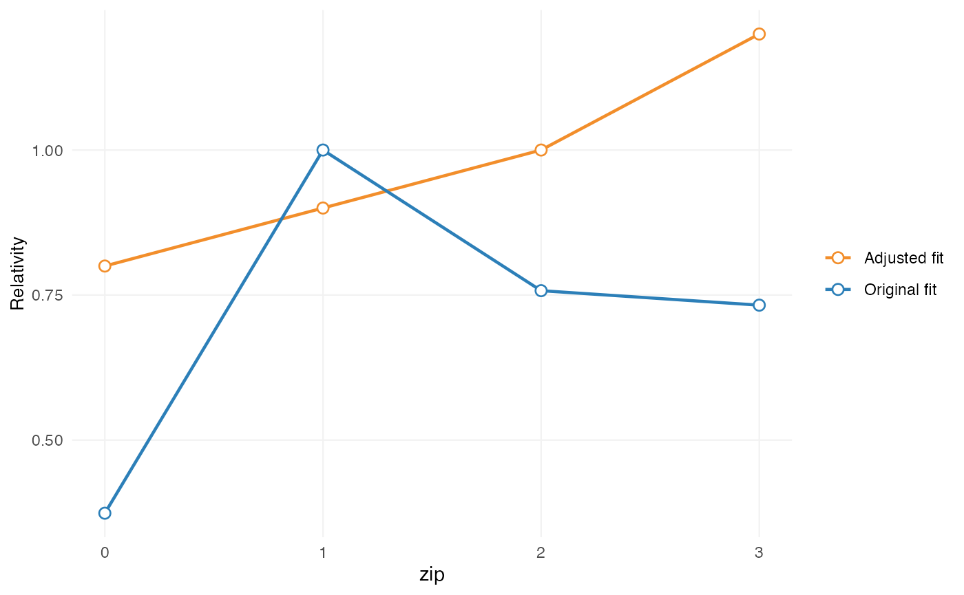

This shows the proposed restricted structure relative to the original fitted model.

Expert-based relativities

Purpose

In some cases, the fitted model uses a broad factor level, while business or portfolio knowledge suggests that more granular differentiation is required.

For example, a model may estimate one coefficient for “construction”, while pricing practice distinguishes between:

residential construction
commercial construction
civil engineering

This is particularly relevant when subgroup exposure is too limited to estimate stable coefficients directly.

Adding relativities


relativities_activity <- relativities_list(
  split_level(
    "construction",
    c("residential_construction", "commercial_construction"),
    c(1.00, 1.15)
  )
)

ref <- ref |>
  add_relativities(
    risk_factor = "business_activity",
    risk_factor_split = "business_activity_split",
    relativities = relativities_activity,
    exposure = "exposure",
    normalize = TRUE
  )

If normalize = TRUE, the relativities are scaled so that their exposure-weighted average remains equal to 1 within the original level.

This preserves the original model signal while introducing finer structure.

Refit

Why refit is required

Refinement steps alter part of the model structure. Once these changes are applied, the remaining coefficients may also need to adjust.

For that reason, the workflow does not end with add_smoothing() or add_restriction(). The final step is:


burn_refined <- refit(ref)

This refits the model while incorporating the refinement steps.

Inspecting the final fitted result

After refit, use rating_table():


rating_table(burn_refined)
#>                risk_factor       level est_burn_refined
#> 1              (Intercept) (Intercept)     9376.5777003
#> 2                  zip_adj           0        0.8000000
#> 3                  zip_adj           1        0.9000000
#> 4                  zip_adj           2        1.0000000
#> 5                  zip_adj           3        1.2000000
#> 6  age_policyholder_smooth     [18,23]        2.3107319
#> 7  age_policyholder_smooth     (23,28]        1.7183044
#> 8  age_policyholder_smooth     (28,33]        1.3763971
#> 9  age_policyholder_smooth     (33,38]        1.2052590
#> 10 age_policyholder_smooth     (38,43]        1.1379656
#> 11 age_policyholder_smooth     (43,48]        1.1204187
#> 12 age_policyholder_smooth     (48,53]        1.1113464
#> 13 age_policyholder_smooth     (53,58]        1.0823030
#> 14 age_policyholder_smooth     (58,63]        1.0176692
#> 15 age_policyholder_smooth     (63,68]        0.9146517
#> 16 age_policyholder_smooth     (68,73]        0.7832839
#> 17 age_policyholder_smooth     (73,78]        0.6464252
#> 18 age_policyholder_smooth     (78,83]        0.5397614
#> 19 age_policyholder_smooth     (83,88]        0.5118045
#> 20 age_policyholder_smooth     (88,93]        0.6238929
#> 21                      bm          bm        0.9976439

At this point, the output no longer represents proposed manual adjustments. It represents the final fitted coefficient structure.

The distinction is:

before refit() –> inspect the refinement plan
after refit() –> inspect the fitted tariff structure

If smoothing, restrictions, and relativities have been applied, they are now embedded in the fitted model output.

Visualising the final structure


rating_table(
  burn_refined,
  model_data = premium_df,
  exposure = "exposure"
) |>
  autoplot()
#> zip_adj, age_policyholder_smooth not in model_data

Model data and rating grids

After refit, model structure can be extracted with model_data():


md <- model_data(burn_refined)
head(md)
#>   age_policyholder age_policyholder_freq_cat_smooth age_policyholder_smooth
#> 1               18                         2.310732                 [18,23]
#> 2               18                         2.310732                 [18,23]
#> 3               18                         2.310732                 [18,23]
#> 4               18                         2.310732                 [18,23]
#> 5               19                         2.310732                 [18,23]
#> 6               19                         2.310732                 [18,23]
#>   nclaims   exposure amount power bm zip age_policyholder_freq_cat
#> 1       1 1.00000000 261777    40  3   3                   [18,25]
#> 2       0 0.09589041      0    68  5   2                   [18,25]
#> 3       0 0.18630137      0    37  3   2                   [18,25]
#> 4       0 0.18904110      0    33  1   2                   [18,25]
#> 5       0 1.00000000      0    47  6   3                   [18,25]
#> 6       1 0.06849315   6642    68  1   3                   [18,25]
#>   pred_nclaims_freq pred_amount_sev   premium zip_adj
#> 1        0.26210740        68671.20 17999.229     1.2
#> 2        0.02502715        70854.51  1773.286     1.0
#> 3        0.04883097        70854.51  3459.894     1.0
#> 4        0.04975980        70854.51  3525.706     1.0
#> 5        0.26044415        68671.20 17885.011     1.2
#> 6        0.01802891        68671.20  1238.067     1.2

Observed model-point combinations can be obtained with rating_grid():


grid <- rating_grid(burn_refined)
head(grid)
#>   zip age_policyholder_smooth bm  exposure count zip_adj
#> 1   1                 (23,28]  1 342.57808   414     1.2
#> 2   1                 (23,28]  2 145.25753   173     1.2
#> 3   1                 (23,28]  3  46.53699    53     1.2
#> 4   1                 (23,28]  4  22.31507    26     1.2
#> 5   1                 (23,28]  5  46.78630    54     1.2
#> 6   1                 (23,28]  6  65.13699    71     1.2
#>   age_policyholder_freq_cat_smooth
#> 1                         2.310732
#> 2                         2.310732
#> 3                         2.310732
#> 4                         2.310732
#> 5                         2.310732
#> 6                         2.310732

This is typically used for:

tariff review
portfolio summaries
compact prediction input
implementation support

Complete example

A full refinement workflow typically looks as follows:


zip_df <- data.frame(
  zip = c(0, 1, 2, 3),
  zip_adj = c(0.8, 0.9, 1.0, 1.2)
)

burn_refined <- prepare_refinement(burn_unrestricted) |>
  add_smoothing(
    x_cut = "age_policyholder_freq_cat",
    x_org = "age_policyholder",
    breaks = seq(18, 95, 5),
    weights = "exposure"
  ) |>
  add_restriction(zip_df) |>
  refit()

rating_table(burn_refined)
#>                risk_factor       level est_burn_refined
#> 1              (Intercept) (Intercept)     9376.5777003
#> 2                  zip_adj           0        0.8000000
#> 3                  zip_adj           1        0.9000000
#> 4                  zip_adj           2        1.0000000
#> 5                  zip_adj           3        1.2000000
#> 6  age_policyholder_smooth     [18,23]        2.3107319
#> 7  age_policyholder_smooth     (23,28]        1.7183044
#> 8  age_policyholder_smooth     (28,33]        1.3763971
#> 9  age_policyholder_smooth     (33,38]        1.2052590
#> 10 age_policyholder_smooth     (38,43]        1.1379656
#> 11 age_policyholder_smooth     (43,48]        1.1204187
#> 12 age_policyholder_smooth     (48,53]        1.1113464
#> 13 age_policyholder_smooth     (53,58]        1.0823030
#> 14 age_policyholder_smooth     (58,63]        1.0176692
#> 15 age_policyholder_smooth     (63,68]        0.9146517
#> 16 age_policyholder_smooth     (68,73]        0.7832839
#> 17 age_policyholder_smooth     (73,78]        0.6464252
#> 18 age_policyholder_smooth     (78,83]        0.5397614
#> 19 age_policyholder_smooth     (83,88]        0.5118045
#> 20 age_policyholder_smooth     (88,93]        0.6238929
#> 21                      bm          bm        0.9976439

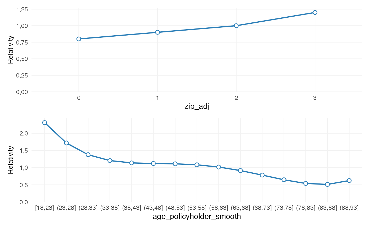
rating_table(
  burn_refined,
  model_data = premium_df,
  exposure = "exposure"
) |>
  autoplot()
#> zip_adj, age_policyholder_smooth not in model_data

Legacy workflow

Legacy entry points remain available:


burn_refined_old <- burn_unrestricted |>
  smooth_coef(
    x_cut = "age_policyholder_freq_man",
    x_org = "age_policyholder",
    breaks = seq(18, 95, 5)
  ) |>
  restrict_coef(zip_df) |>
  refit_glm()

These are primarily maintained for backward compatibility.

For new code, the standard workflow is:


prepare_refinement() |> add_*() |> refit()

This makes the sequence of tariff adjustments explicit and improves interpretability, governance, and auditability.

Summary

The refinement workflow separates:

model estimation
tariff adjustments
final fitted output

This makes it possible to move from a raw GLM to a tariff structure that is:

statistically grounded
interpretable
commercially usable
easier to implement

Next steps

For the underlying pricing concepts, see:

Pricing principles

For the standard workflow from portfolio analysis to fitted tariff, see:

Getting started

Introduction

When refinement is used

Example setup

The refinement object

Smoothing

Purpose

Adding smoothing

Inspecting smoothing before refit

Choosing a smoothing method

Restrictions

Purpose

Adding restrictions

Inspecting restrictions before refit

Expert-based relativities

Purpose

Adding relativities

Refit

Why refit is required

Inspecting the final fitted result

Visualising the final structure

Model data and rating grids

Complete example

Legacy workflow

Summary

Next steps